Translating between the dispersion term in a negative binomial regression and random variables in SPSS

When estimating a negative binomial regression equation in SPSS, it returns the dispersion parameter in the form of:

Var(x) = mean + mean*dispersion

So a dispersion parameter of 0 in this notation is the same as a variable that is Poisson distributed without any extra dispersion. When generating random variables from the negative binomial distribution, SPSS does not take the parameters like this, but the more usual N trials with P successes. Stealing a bit from the R documentation for dnbinom, I was able to translate between the two with just a tedious set of algebra. So with our original distribution being:

Mean = mu
Variance = mu + mu*a

R has an alternative representation closer to SPSS’s based on:

Mean = mu
Variance = mu + mu^2/x

Some algebra will reveal that in this notation x = mu/a. Also, R’s help for dbinom states that in the original N and P notation that p = x/(x + mu). So here with mu and a (again a is the dispersion term as reported by GENLIN in SPSS) we can solve for p.

x = mu/a
p = (mu/a)/(mu/a + mu)

And since p is solved, R lists the mean of the distribution in the N and P notation as:

n*(1-p)/p = mu

So with p solved we can figure out N as equal to:

mu*p/(1-p) = n

So to reiterate, if you have a mean of 1 and dispersion parameter of 4, the resultant N and P notation would be:

p = (mu/a)/(mu/a + mu) = (1/4)/(1/4 + 1) = 1/5
n = mu*p/(1-p) = 1*0.2/(1 - 0.2) = 1/4

Here we can see that in the N and P notation the similar negative binomial model results in a fractional number of successes, which might be a surprising result for some that it is even a possibility. (There is likely an easier way to do this translation, but forgive me I am not a mathematician!)

Now we would be finished, but unfortunately SPSS’s negative binomial random functions do not take values of N less than 1 (R’s dnbinom does). In the case N is greater than 1 the NEGBIN functions (CDF, PDF and RV) will work (and will take fractional values over 1). But if N is smaller than 1, we have to do another translation of the N and P notation to the gamma distribution to be able to draw random numbers in SPSS. Another representation of the negative binomial model is a mixture of Poisson distributions, with the distribution of the mixtures being from a gamma distribution. Wikipedia lists a translation from the N and P notation to a gamma with shape = N and scale = P/(1-P).

So I wrapped these computations up in an SPSS macros that takes the mean and the dispersion parameter, calculates N and P under the hood, and then draws a random variable from the associated negative binomial distribution.

*Type can either be CDF, PDF or RV.
DEFINE !NegBinRV (mu = !TOKENS(1)
       /disp = !TOKENS(1)
       /out = !TOKENS(1) )
COMPUTE #x = !mu/!disp.
COMPUTE #p = #x / (#x + !mu).
COMPUTE #n = #p / (1 - #p).
COMPUTE #G = RV.GAMMA(#n,#p/(1 - #p)).
COMPUTE !Out = RV.POISSON(#G).
!ENDDEFINE.

I am not sure if it is possible to use this gamma representation and native SPSS functions to calculate the corresponding CDF and PDF of the negative binomial distribution. But we can use R to do that. Here is an example of keeping the mean at 1 and varying the dispersion parameter between 0 and 5.

BEGIN PROGRAM R.
library(ggplot2)
x <- expand.grid(0:10,1:5)
names(x) <- c("Int","Disp")
mu <- 1
x$PDF <- mapply(dnbinom, x=x$Int, size=mu/x$Disp, mu=mu)
#add in poisson
t <- data.frame(cbind(0:10,rep(0,11),dpois(0:10,lambda=1)))
names(t) <- c("Int","Disp","PDF")
x <- rbind(t,x)
p <- ggplot(data = x, aes(x = Int, y = PDF, group = as.factor(Disp))) + geom_line()
p
#for the CDF
x$CDF <- ave(x$PDF, x$Disp, FUN = cumsum)
END PROGRAM.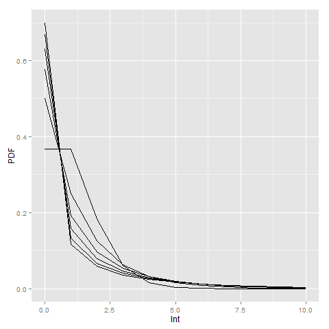

Here you can see how the larger dispersion term can easily approximate the zero inflation typical in criminal justice data (see an applied example from my work). R will not take a dispersion parameter of zero in this notation (as the size would be divided by zero and not defined), so I just tacked on the Poisson distribution with a mean of zero.

Here is an example of generating random data from a negative binomial distribution with a mean of 1 and a dispersion parameter of 4. I then grab the PDF from R, and superimpose them both on a chart in SPSS (or perhaps I should call it a PMF, since it only has support on integer values). You can see the simulation with 10,000 observations is a near perfect fit (so a good sign I did not make any mistakes!)

*Simulation In SPSS.
INPUT PROGRAM.
LOOP Id = 1 TO 10000.
END CASE.
END LOOP.
END FILE.
END INPUT PROGRAM.
DATASET NAME RandNB.

!NegBinRV mu = 1 disp = 4 out = NB.

*Making seperate R dataset of PDF.
BEGIN PROGRAM R.
mu <- 1
disp <- 4
x <- 0:11
pdf <- dnbinom(x=x,size=mu/disp,mu=mu)
#add in larger than 10
pdf[max(x)+1] <- 1 - sum(pdf[-(max(x)+1)])
MyDf <- data.frame(cbind(x,pdf))
END PROGRAM.
EXECUTE.
STATS GET R FILE=* /GET DATAFRAME=MyDf DATASET=PDF_NB.
DATASET ACTIVATE PDF_NB.
FORMATS x (F2.0).
VALUE LABELS x 11 '11 or More'.

*Now superimposing bar plot and PDF from separate datasets.
DATASET ACTIVATE RandNB.
RECODE NB (11 THRU HIGHEST = 11)(ELSE = COPY) INTO NB_Cat.
FORMATS NB_Cat (F2.0).
VALUE LABELS NB_Cat 11 '11 or More'.

GGRAPH
  /GRAPHDATASET NAME="Data" DATASET='RandNB' VARIABLES=NB_Cat[LEVEL=ORDINAL] COUNT()[name="COUNT"]
  /GRAPHDATASET NAME="PDF" DATASET='PDF_NB' VARIABLES=x pdf
  /GRAPHSPEC SOURCE=INLINE.
BEGIN GPL
  SOURCE: Data=userSource(id("Data"))
  DATA: NB_Cat=col(source(Data), name("NB_Cat"), unit.category())
  DATA: COUNT=col(source(Data), name("COUNT"))
  SOURCE: PDF=userSource(id("PDF"))
  DATA: x=col(source(PDF), name("x"), unit.category())
  DATA: den=col(source(PDF), name("pdf"))
  TRANS: den_per = eval(den*100)
  GUIDE: axis(dim(1))
  GUIDE: axis(dim(2))
  SCALE: linear(dim(2), include(0))
  ELEMENT: interval(position(summary.percent(NB_Cat*COUNT)), shape.interior(shape.square))
  ELEMENT: point(position(x*den_per), color.interior(color.black), size(size."8"))
END GPL.